Optical Encoder Long Cable Runs: Signal Integrity, Drivers, Termination, and Cabling for Extended Distances
Moving encoder electronics away from the readhead is the most common way to protect them from the machine—but every meter of cable attenuates, delays, and distorts the position signal. This guide explains what cable length does to analog sine and differential digital encoder signals, how to size drivers, repeaters, and termination for the run, how to specify cable, connectors, and shielding for a precision axis, and how to qualify and diagnose a long-distance installation so the count arriving at the controller is as clean as the count that left the readhead.
Published
DIRECT ANSWER
What should a buyer prioritize?
A long encoder cable run changes the signal before it reaches the controller: cable capacitance slows digital edges and introduces duty-cycle distortion, resistance and attenuation reduce analog amplitude into the interpolation floor, shield and ground potential differences inject noise into the count, and propagation delay eats into the timing budget of serial absolute protocols. A readhead that produces a clean quadrature pair on a one-meter bench cable can deliver shifted, asymmetrical, or intermittently miscounting signals at fifteen meters—especially at the high edge frequencies that fast stages produce.
The engineering response is to treat distance as a specified interface, not an afterthought: keep the analog front end and interpolation close to the readhead wherever possible, transmit differential signals (line-driver TTL or sinusoidal 1 Vpp on twisted pairs) through cable whose capacitance and impedance the supplier's length-versus-speed data assumes, terminate receivers correctly, use repeaters or remote electronics boxes when runs exceed what a direct drive supports, route and ground the shield deliberately, and qualify the installed run with signal measurements at the receiver end under real motion. The supplier's published maximum cable length is valid only for the cable type, termination, and grounding discipline it was measured with.
ENGINEERING CONTEXT
The decision starts with the real constraint.
Long encoder cable runs are usually created by a well-intentioned architectural decision: put the interpolation and counting electronics in the clean, accessible cabinet, and let only the sensor live on the machine. What gets underestimated is how hostile the intervening meters are to a precision signal. Cable capacitance—typically around 100 pF per meter for shielded cable—combines with driver output impedance to slow every edge, and because the two channels rarely degrade identically, the quadrature relationship drifts toward duty-cycle distortion that interpolation converts into periodic position error. Analog sine signals lose amplitude into cable resistance and capacitance until they sit near the interpolation threshold, where noise starts producing spurious counts. Ground potential differences between machine base and electronics cabinet drive current through the shield. Intermediate connectors and drag-chain flexing add intermittent contacts that look exactly like firmware faults. Worst of all, the system often works at commissioning: the failures appear weeks later at higher speeds, higher duty cycles, or in a different season's temperature, by which time the cable run has been buried in the machine and nobody wants to believe it is the cause.
The required cable length, the maximum stage velocity, the encoder resolution, and therefore the worst-case edge frequency written down together, and checked against the supplier's length-versus-frequency data for the exact interface and cable type—before hardware is ordered.
02
Cable specified as part of the interface
Capacitance per meter, characteristic impedance, twisted-pair construction, shield coverage, conductor gauge, and flex rating matched to the encoder interface specification and the machine's cable path, with no undocumented substitutions during installation.
03
Termination, grounding, and routing plan
Receiver termination values per the interface standard, a defined shield-grounding scheme at machine and cabinet ends, physical separation from motor drives and switching power, and a single grounding architecture for the whole signal chain.
04
Signal qualification at the receiver end
Amplitude, edge rates, quadrature symmetry, and count stability measured at the controller end of the installed run, under maximum speed and after temperature stabilization, and recorded as the baseline for future troubleshooting.
BUYER MATRIX
Compare evidence, not feature labels.
Give every shortlisted supplier the same process definition and request configuration-specific proof.
Signal interface options for long encoder cable runs compared
Aspect
Analog 1 Vpp sine run to remote interpolation
Differential line-driver TTL (RS-422 style)
Remote electronics box / repeater at mid-run
Distance behavior
Amplitude rolls off with cable capacitance and resistance; edge steepness not critical, but signal can sink toward the interpolation threshold on long runs
Capacitance slows edges and erodes quadrature symmetry; practical limit typically tens of meters with low-capacitance cable and correct termination
Analog or short digital segment to the box, then a regenerated driver signal onward; effectively extends the limit by relocating the electrical source
Speed ceiling
Set by interpolation electronics and signal amplitude, not by edge rate; tolerant of long cable at moderate speed
Set by edge frequency versus degraded rise time at the receiver; the combination of speed, resolution, and length must be checked jointly
Restores clean edges downstream of the box, so the long run no longer limits the achievable counting frequency
Failure modes
Slow amplitude loss with temperature and aging; noise near threshold produces sporadic miscounts that are hard to reproduce
Duty-cycle distortion and marginal edges; intermittent loss under vibration at connectors; sensitive to missing termination
The repeater or box becomes an active component with its own power and reliability; failures localize downstream of it
Best use
Moderate distances where the readhead's analog signal is strong and interpolation can sit in the cabinet; common on machine tools
Standard choice for direct digital runs within the supplier's rated length at the planned speed
Long runs, high speeds, or one encoder feeding multiple consumers; the standard architecture for large machines
What cable length actually does to a position signal
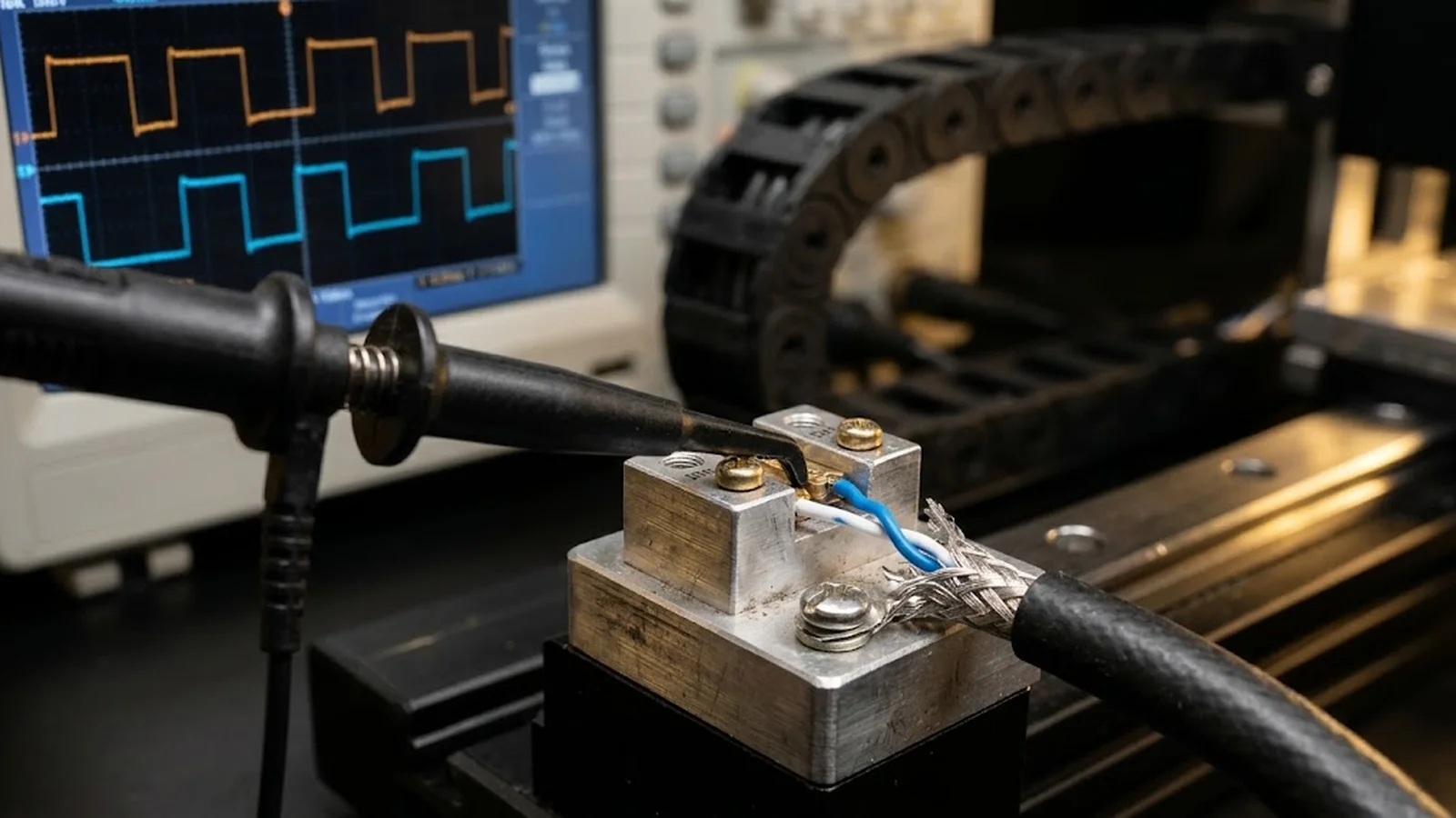
An encoder cable is not a passive extension cord; it is an RC network and an antenna wrapped around the signal. Every meter adds series resistance and shunt capacitance—roughly 100 picofarads per meter is typical for shielded instrumentation cable—so the driver, designed to produce crisp edges into a short bench load, now charges and discharges a substantial capacitance through its own output impedance. For an analog sine signal the consequences are gentle: amplitude falls, phase shifts slightly, and the waveform stays sinusoidal. For a square-wave quadrature signal the consequences are structural: rise and fall times stretch from nanoseconds toward tenths of a microsecond, and because the two channels and their two directions of travel rarely degrade identically, the quadrature phase relationship skews. The interpolation electronics, which assume clean 90-degree spacing, convert that skew into duty-cycle error and periodic position ripple. Long runs are created for good reasons—electronics must live somewhere clean, serviceable, and thermally stable—but the distance that protects the electronics taxes the signal, and the tax scales with every meter and every edge frequency the machine demands.
Distance also multiplies exposure. The longer the cable, the more capacitively and inductively coupled noise it collects from servo drives, switching supplies, and contactors along its path, and the larger the ground-potential difference between the machine base where the readhead lives and the cabinet where the counting electronics sit. None of these effects is dramatic on an oscilloscope at rest—which is why bench checks pass—but they accumulate exactly where the machine operates hardest: at speed, under load, over temperature. This is also why maximum velocity must be judged with the whole signal chain in mind, not from the readhead datasheet alone, as the frequency-limit logic in the [guide to encoder high-speed counting and frequency limits](/technology/optical-encoder-high-speed-counting-frequency-limits-guide/) makes explicit for the counting stage that sits at the end of your cable.
The electrical limits: capacitance, edge rate, and amplitude
Two numbers govern a digital run. The first is the RC time constant formed by cable capacitance and the driving impedance: a line driver with 50 ohms of output impedance driving 15 meters at 100 pF/m faces 1.5 nanofarads, giving a time constant near 75 nanoseconds and rise times in the hundreds of nanoseconds once the receiver threshold is reached. The second number is the edge frequency the machine needs: velocity times counts per revolution or per meter, halved for the two edges if the receiver counts both. When edge period approaches the degraded rise time, the signal crosses the receiver threshold late and asymmetrically, quadrature margins collapse, and miscounts begin exactly at maximum speed—the one condition acceptance tests sometimes forget to exercise. Characteristic impedance and propagation delay complete the picture: an unterminated pair reflects energy back down the cable, and reflections that arrive during a slow edge can cross the receiver threshold twice, which the counter experiences as phantom steps. The remedy is arithmetic before purchase: derive the worst-case edge frequency from the motion profile, obtain the supplier's cable-length-versus-frequency curve for the specific interface, and keep the planned run inside it with margin for cable substitutions and aging.
For analog runs the governing quantities are amplitude and noise margin. A 1 Vpp sinusoidal signal attenuates slowly over tens of meters, but the interpolation electronics need a minimum amplitude and a minimum signal-to-noise ratio to subdivide cleanly; a run that delivers 600 millivolts peak into a noisy cabinet is worse than a shorter run delivering 950, because subdivision quality degrades with noise margin long before the signal disappears outright. DC resistance matters too, particularly for the readhead's supply lines—a 20-meter run on thin conductors can drop the readhead supply below its regulated minimum, shrinking signal amplitude at the source before the signal ever travels. Voltage-drop calculation for supply, DC feedback lines, and signal amplitude belongs in the run design, and where the interface choice is between keeping analog all the way to the cabinet or converting to a differential digital signal at the readhead, the trade-offs in level, edge rate, and receiver expectations are detailed in the [guide to TTL and line driver output interfaces](/technology/optical-encoder-ttl-line-driver-output-interface-guide/).
Interface architecture for distance: drivers, repeaters, and remote electronics
The cleanest long-run architecture keeps the analog front end—photodiode amplifiers, gain adjustment, interpolation—physically close to the readhead, and transmits robust signals onward. That closeness takes one of two forms. In the first, the readhead itself contains a line driver and outputs differential digital quadrature (RS-422 style) or a serial absolute protocol; the cable then carries a signal designed for distance. In the second, an intermediate electronics box—sometimes called a repeater, pulse shaper, or remote interpolation unit—mounts on the machine within a short analog reach of the readhead, restores the signal to full amplitude and defined edges, and drives the long run to the cabinet. In both cases the sensitive analog circuitry sees only the short, benign segment it was designed for, and the harsh electrical environment of the long run sees only robust signals. Both forms share the same principle: never ask a marginal signal to survive meters it was not designed for when a regenerative stage can sit at the boundary between machine and distance. Where the goal is instead to distribute one encoder to several controllers—a motion controller plus a verification system, for example—the splitter architecture belongs to the same family of decisions, because each added consumer loads the driver and shortens the distance the signal can still reach.
Choosing among direct analog, direct line driver, and repeater architectures is a function of run length, edge frequency, and environment. Direct analog to the cabinet is reasonable for moderate lengths and moderate speeds; differential line driver is the default for runs of a few meters to a few tens of meters provided termination and cable are right; repeaters and remote boxes are the standard answer for machine tools and large gantries where runs reach 25, 50, or more meters or where one encoder must feed several controllers through a splitter. Serial absolute interfaces add their own constraint: protocols such as BiSS-C and EnDat specify maximum cable lengths that depend on clock frequency, and the propagation delay of a long run consumes the protocol's timing budget just as surely as a slow receiver does—the coupling between cable, clock rate, and frame timing is covered in the [guide to encoder interface protocols including BiSS and EnDat](/technology/optical-encoder-interface-protocols-biss-endat-guide/).
Cable, connectors, termination, and grounding practice
The cable is a precision component and should be bought like one, with a part number, a specification, and a record of what was actually installed. The encoder supplier's length ratings assume a cable class: individually shielded twisted pairs for each differential signal, overall shield with high coverage, capacitance at or below the assumed figure, conductor gauge adequate for supply voltage drop at full run length, and an outer jacket suited to the machine's cable path. Substituting a generic shielded cable with double the capacitance silently halves the rated distance. Temperature rating matters as well: cable routed near drives or through hot machine zones must tolerate the ambient it actually sees, and its insulation capacitance shifts with temperature in ways the length rating already absorbed only if the cable class matches the specification. Connectors deserve equal respect: every intermediate connector is a reflection point, a corrosion site, and a vibration failure candidate, so runs should be continuous where possible, and where a break is unavoidable it should use qualified circular connectors with secured couplings and strain relief that carries load on the jacket, not the conductors.
Termination and grounding complete the chain. Differential receivers should be terminated per the interface standard—typically a resistor across each pair at the receiver input, sized to the cable's characteristic impedance class—because an unterminated long pair rings, and ring crossings near the threshold become false counts at speed. The shield should be terminated according to a deliberate scheme: grounded at the cabinet end as a minimum, and bonded at both ends when the measurement shows ground-potential differences are small, since a floating shield stops shielding above its own capacitance to ground. And routing is half of signal integrity: encoder cable belongs separated from motor power and braking resistor leads, crossing them at right angles where crossing is unavoidable, out of shared glands and trays with switching loads. The full discipline—separation distances, tray practice, and shield-bonding decisions—is consolidated in the [guide to EMC, cable routing, and grounding](/technology/encoder-emc-cable-routing-grounding-guide/), and where the run travels through a moving chain, the mechanical side of the same cable is governed by the drag-chain flex-life rules in the [encoder cable flex and drag chain guide](/technology/optical-encoder-cable-flex-life-drag-chain-guide/).
Buy cable to the interface specification: per-meter capacitance, twisted pairs with individual shields, conductor gauge sized for supply drop at full length
Terminate every differential pair at the receiver per the interface standard; verify termination presence during commissioning, not after failures
Decide the shield-grounding scheme from measurement—one end as default, both ends where potential differences allow—and write it down
Minimize intermediate connectors; where unavoidable, use qualified circular connectors with jacket-borne strain relief
Keep encoder cable separated from motor drives, contactors, and switch-mode supplies; cross at right angles where paths must meet
Qualifying and diagnosing the installed long run
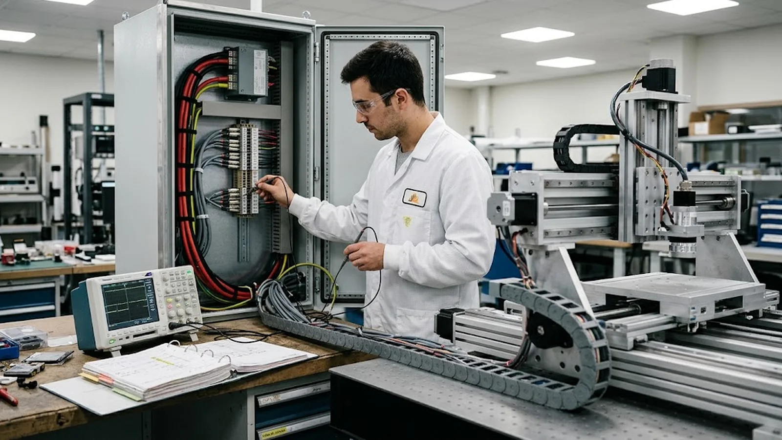
Qualification of a long cable run happens at the receiver end, under motion, after thermal stabilization. The measurement set is compact: amplitude of each differential signal at the controller input, rise and fall times compared between channels, quadrature symmetry read as duty cycle with a counter or scope, and common-mode noise with the stage servoing. Then the dynamic test: the stage run at maximum velocity through full travel while a diagnostic counts error or lost-step indications, repeated after the machine has been at operating temperature for an hour, because marginal amplitude and slow edges worsen with temperature exactly when duty cycles are heaviest. A run that passes at cold-start and fails warm is not a curiosity; it is the signature of an amplitude or termination margin that was thin from the beginning and was used up by thermal drift. Recording these numbers as the run's baseline is what makes future diagnosis rational—the difference between 'the signal looks wrong' and 'the rise time degraded from 90 to 180 nanoseconds since acceptance' is the difference between a week of guessing and an afternoon of cable-end measurements. For machines that run for years, a short re-verification of these same parameters at every major service keeps the baseline honest against connector aging, shield corrosion, and cable replacements made in the meantime.
Diagnosis of a run that miscounts follows the same geometry. Localize first: move the measurement point to the readhead end of the cable—if the signal is already degraded there, the problem is the readhead or its supply; if it is clean at the source and dirty at the receiver, the run is the suspect. Within the run, the usual suspects arrive in order: a missing or wrong termination, an intermediate connector working loose under vibration, a shield grounded at neither end or at three, a cable substituted during maintenance with a higher-capacitance type, and heat where the run passes near a drive. The systematic versions of these measurements—Lissajous figures for analog chains, quadrature timing for digital ones—are laid out in the [guide to signal quality and distortion troubleshooting](/technology/linear-encoder-signal-quality-distortion-troubleshooting-guide/), and working through them at both cable ends resolves the great majority of long-run faults without replacing a single healthy component.
CONCLUSION
Design the distance into the interface, and the cable stops being a risk.
A long encoder cable run fails in predictable ways: capacitance-slowed edges that erode quadrature margins, attenuated analog signals that sink toward the interpolation threshold, unterminated pairs that ring into false counts, and shields that route noise instead of draining it. Every one of these is decided at design time, not at troubleshooting time—by keeping the analog front end close to the readhead, choosing a driver or repeater architecture matched to the run length and edge frequency, buying cable to the interface specification, and routing and grounding the run as deliberately as any other precision signal.
The qualification habit that separates reliable installations from intermittent ones is small: measure amplitude, edge times, and symmetry at the receiver end of the installed run, at speed and at temperature, and keep those numbers with the machine's file. When the axis later miscounts, those baselines turn a mysterious intermittent fault into a measurable degradation with a location—and an afternoon fix.
Length-versus-frequency data from the encoder supplier for the exact interface, cable type, and termination used, with the planned run length inside it
Cable specification sheet: capacitance per meter, characteristic impedance, shield coverage, conductor gauge, and flex-cycle rating for the installed cable path
Receiver-end signal measurements on the installed run: amplitude, rise time, quadrature symmetry (duty cycle), and common-mode noise, at maximum stage speed
Count stability and position repeatability over the full travel at operating speed, recorded after temperature stabilization, as the acceptance baseline
Shield-grounding and routing record: where the shield is terminated, what the cable is separated from, and any intermediate connectors with their strain relief
FAQ
Questions engineers ask before selection.
What is the maximum cable length for an encoder signal?
There is no universal number; the limit is set jointly by the interface (analog sine, line-driver TTL, or serial absolute protocol), the cable's capacitance and resistance per meter, the termination, and the edge frequency your machine's speed and resolution demand. Suppliers publish length-versus-frequency data for defined cable classes—use the curve for your exact configuration with margin, rather than a catalog headline figure.
Can analog sine signals travel farther than TTL square waves?
Often yes, over moderate distances, because sine signals have no fast edges to slow down—their amplitude rolls off gently and interpolation tolerates small phase shifts. The trade-off is that a degraded sine can drift near the interpolation threshold, where noise causes sporadic miscounts. For long runs at high speed, the usual answer is a differential digital signal from the readhead or a repeater at mid-run, not an extended analog run.
When do I need a repeater or remote electronics box?
When the planned run exceeds the supplier's direct-drive rating for your speed and cable, when supply voltage drop becomes significant, or when one encoder must feed multiple controllers. The box sits within the short reach the analog signal can manage, restores full amplitude and defined edges, and drives the long run with a fresh, specified signal—turning one marginal long path into one short segment plus one robust segment.
Should the encoder cable shield be grounded at one end or both?
One end is the conservative default because it breaks the ground loop that machine-to-cabinet potential differences would otherwise drive through the shield. Both-end bonding shields high frequencies better and is appropriate when measurements confirm small potential differences and a grounding architecture that limits loop current. Decide from measurement, document the decision, and never leave a shield floating at both ends.
The axis miscounts only at maximum speed—where do I start?
Speed-dependent miscounts point at edge integrity. Measure rise and fall times and quadrature duty cycle at the receiver end of the cable at rest, then compare with the acceptance baseline and the supplier's limits. Check that termination is present and correct, that no cable was substituted with a higher-capacitance type, and that connectors are tight. If the signal is already degraded at the readhead end, the cable is exonerated and the readhead or its supply becomes the suspect.