
Simultaneous 2D measurement
Error measured on both axes at the working point while both axes move, using a grid encoder, 2D interferometry or an equivalent calibrated reference—not single-axis tests extrapolated.
TECHNOLOGY / STAGE METROLOGY
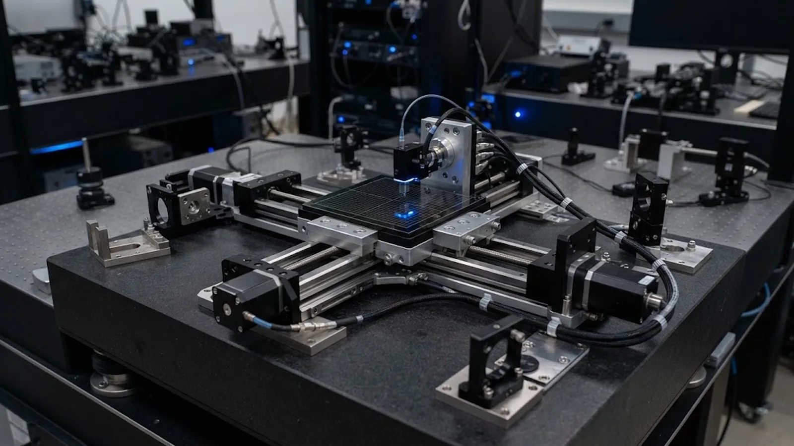
Commanding X and watching Y move is the defining symptom of cross-coupling error. This guide explains where XY cross-coupling comes from in precision stages, how to measure it with grid encoders, circle tests and laser vector methods, and how to specify and mitigate it in a multi-axis system.
Published
DIRECT ANSWER
Cross-coupling error is the motion error that appears on one axis when another axis is commanded. In an ideal XY stage, moving X leaves Y untouched; in a real one, Y sees a parasitic displacement or rotation composed of geometric contributions—straightness error of each axis, squareness error between them, Abbe offsets—and control contributions, where dual-axis drives or imperfect decoupling push correction forces into the wrong axis. The result shows up directly as contouring error: a circle programmed on the axes comes out elliptical or tilted, and scanned trajectories carry systematic cross-tracks.
Measurement needs instruments that watch both axes simultaneously: a calibrated two-dimensional grid encoder reports X and Y error at the tool point during motion, dynamic circle tests expose coupling as shape distortion at process speed, and laser vector or straightness measurements attribute the coupling to specific axes. Mitigation is layered—mechanical (improve straightness and squareness, reduce Abbe offsets), geometric (map and compensate squareness and cross-track in the controller) and control-side (decoupling and cross-coupling gains)—and each layer should be verified with the same 2D measurement that found the error.
ENGINEERING CONTEXT
Single-axis specifications look impeccable: X positioning accuracy certified with a laser interferometer, Y likewise, both within nanometres. Then a diagonal scan, a circular trajectory or a raster with flyback shows errors several times larger, purely in the combination of axes. The culprit is cross-coupling—every axis certification was taken with only one axis moving, so the interaction terms were invisible. Straightness error of the X carriage displaces Y; an 80-microradian squareness error displaces Y by 80 nanometres per millimetre of X travel; dual-drive control loops fight each other at direction reversals. None of these appear on a single-axis report, yet they dominate every multi-axis process: raster scanning, stitching, wafer mapping and contour following all live exactly where the coupling lives.
Discuss your requirement ↗CRITICAL REQUIREMENTS
Error measured on both axes at the working point while both axes move, using a grid encoder, 2D interferometry or an equivalent calibrated reference—not single-axis tests extrapolated.
Straightness per axis, squareness between axes and Abbe offsets measured and reported as separate line items, so coupling can be attributed and compensated.
Coupling evaluated during representative trajectories—rasters, circles, direction reversals—at production velocity, since control-induced coupling is speed- and acceleration-dependent.
Squareness and cross-coupling compensations documented, and their effect verified with the same 2D measurement after application, with residual contouring error stated.
BUYER MATRIX
Give every shortlisted supplier the same process definition and request configuration-specific proof.
| Source | Signature | Measured by | Primary mitigation |
|---|---|---|---|
| Axis straightness error | Y displacement proportional to X position, periodic with carriage travel | Straightness interferometer or artifact; 2D grid encoder | Mechanical improvement, then cross-track error map compensation |
| Squareness between axes | Y error growing linearly with X travel; tilted trajectories | Squareness straightedge, optical square or reversal; grid encoder area map | Squareness compensation in controller; mechanical realignment if severe |
| Abbe offsets with angular error | Coupling that grows with angular error of the moving carriage | Angular metrology plus offset measurement | Reduce offsets toward the tool point; correct angular terms |
| Dual-drive / gantry control conflict | Error spikes at direction reversal or high acceleration; oscillation at drive modes | Dynamic circle test; synchronized 2D capture at speed | Cross-coupling control gains, synchronized dual-axis tuning |
| Guideway wear or contamination | Coupling that drifts over time and varies along travel | Periodic 2D remapping against the baseline | Maintenance schedule plus periodic remap |
| Foundation and thermal asymmetry | Slowly changing squareness with temperature drift | Squareness re-measurement across thermal states | Thermal control, symmetric structures, warmup procedure |
Cross-coupling is defined at the point that matters—the tool, sensor or beam spot. When X is commanded, the working point should move only along X; its parasitic motion along Y and in rotation is cross-coupling error. The geometric part decomposes neatly: the X carriage's straightness error moves the point sideways, any squareness error between the axes makes X travel lean into Y by a fixed angle, and Abbe offsets convert the carriage's roll, pitch and yaw into lateral displacement. These terms are quasi-static, repeatable and therefore compensable.
The control part is less polite. Multi-axis machines with dual drives, gantry configurations or coordinated trajectories couple through the controller: each axis loop sees disturbance forces from the others, and imperfect decoupling means accelerating X kicks Y, most visibly at reversals and high acceleration. This component is velocity- and tuning-dependent, so it must be measured under representative motion rather than inferred from static geometry. A stage can have perfect geometric squareness and still contour poorly because its loops fight at every corner.
The defining measurement discipline is simultaneity: both axes' errors captured at the tool point while motion happens. A calibrated two-dimensional grid encoder is the reference of choice—it reads X and Y displacement continuously at high bandwidth across its calibrated area, producing a map in which straightness coupling appears as cross-track deviation, squareness as a systematic tilt that grows with travel, and control coupling as distortion concentrated at reversals and corners. Circle tests compress the same information into one shape: a perfect circle command returns an ellipse from squareness, a tilted ellipse from cross-axis offset, and lobed distortion from control coupling at reversal points.
Attribution then needs the per-axis record. Straightness and angular measurements on each axis alone, taken in the same campaign, let the 2D map be decomposed into causes. The practical sequence is: map in 2D, measure per-axis geometry, apply compensation—squareness constant, cross-track map, control decoupling gains—then remap in 2D and state the residual contouring error. Compensation that is never re-verified in 2D is a guess with a parameter file.
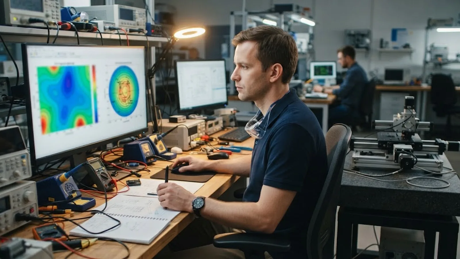
Modern controllers absorb a remarkable share of cross-coupling: squareness constants correct the fixed axis-to-axis angle, cross-track error maps cancel straightness-induced coupling over travel, and decoupling control terms reduce dynamic interaction between loops. Applied well, a stage with micrometre-scale raw geometric coupling can contour at sub-micrometre levels. The discipline is to treat compensation as a layer over measured mechanics, not a substitute for them: compensations are valid only over the travel and conditions where they were mapped, they add parameters that can be mis-set, and they cannot follow mechanical drift they were never re-measured against.
Two habits keep the layer honest. First, version and date every compensation table, and tie each re-measurement campaign to the table version active during it—when a stage's behavior changes months later, the baseline answers whether the mechanics moved or the parameters did. Second, watch the thermal boundary: squareness is a property of a structure at a temperature, and a machine that maps beautifully at 20 degrees can couple differently at 22. Specification of the thermal state belongs with the squareness number.
A single-axis accuracy clause cannot buy contouring quality. A useful multi-axis specification adds: squareness between axes with method and uncertainty; straightness and angular error per axis; a 2D error map over the working area from a grid encoder or equivalent; residual contouring error at a defined trajectory and speed, measured after compensation; and the compensation state, documented, that produced the result. For scanning applications, add the coupling behavior during constant-velocity raster segments and at flyback, since those are where the process spends its time.
The payoff is measured in process terms: stitched fields land on each other, rasters keep their pitch across the full scan, and circles stay round. Machines qualified only axis-by-axis deliver all of these poorly, and the deficiency surfaces exactly where the work is—on the diagonal. Multi-axis performance is a property of the pair of axes and their control, and it should be specified, measured and accepted as such.
CONCLUSION
Cross-coupling error lives in the interaction that single-axis certification never exercises: straightness of one axis displacing another, squareness leaning every diagonal trajectory, Abbe offsets converting tilt to lateral error, and control loops interfering at reversals. For any process that scans, stitches or follows contours, these interaction terms dominate the accuracy that the individual axis certificates promise.
Specify and verify the system as a system: simultaneous two-dimensional measurement at the tool point, per-axis geometry for attribution, compensation applied and then re-verified in 2D with residuals stated, and thermal and compensation states documented with every campaign. Contouring quality is bought with this evidence—not with two good single-axis reports.
EVIDENCE CHECKLIST
FAQ
The parasitic motion that appears on one axis when another is commanded, evaluated at the working point. It combines geometric sources—straightness error of each axis, squareness between axes, Abbe offsets—with control-side coupling between axis loops, and it appears directly as contouring and cross-track error in multi-axis trajectories.
Linearly with travel: a squareness error of one microradian displaces the working point by one nanometre per millimetre of travel on the other axis, so 80 microradians—about 17 arcseconds—yields 80 nanometres of cross-error per millimetre. Over a 300-millimetre travel, that is 24 micrometres before any compensation.
Single-axis tests move one axis at a time, so interaction terms never activate. Cross-coupling appears only during combined motion, and control-induced coupling additionally depends on velocity and acceleration. A circle or raster test at process speed exposes what the individual axis certificates cannot see.
A calibrated two-dimensional grid encoder is the strongest general tool: it captures X and Y error simultaneously at the tool point with high bandwidth across the working area. Dynamic circle tests are an excellent fast screen, while laser straightness and squareness measurements provide the per-axis attribution needed to assign causes.
It can remove a large, repeatable share—squareness constants and cross-track maps handle the geometric terms, decoupling gains reduce dynamic interaction. What remains is whatever drifted after mapping, plus terms outside the mapped conditions. Compensation must be re-verified in 2D after any mechanical, thermal or parameter change.
Travel ranges, the trajectory types and speeds your process uses, the contouring or overlay tolerance, and any existing axis certification reports. SENFU can help define the 2D measurement plan, squareness specification and compensation verification for the application.
AUTHORITATIVE SOURCES
TECHNICAL REVIEW
Send the application, critical parameters and any drawing or process information available.
Discuss your application ↗