
Reference measurement
A calibrated, traceable measuring device—typically a laser interferometer or a comparator system—used along the same axis as the encoder.
TECHNOLOGY / ENCODER ACCURACY
Learn how linear encoder error maps are measured with a reference standard, how linear and multipoint compensation work, and what error remains after compensation.
Published
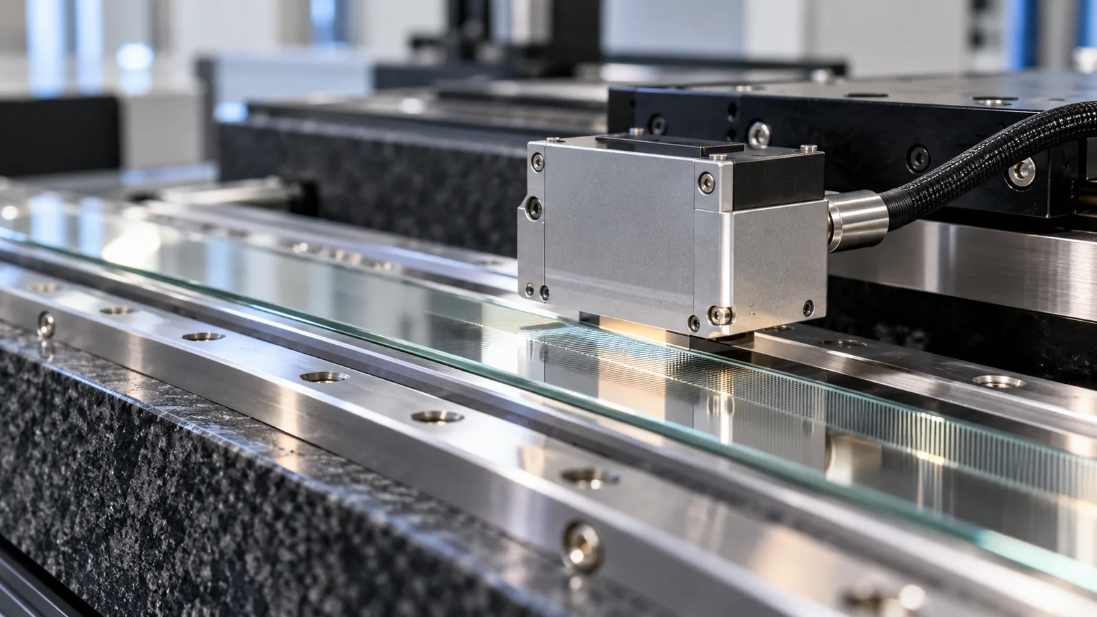
DIRECT ANSWER
Encoder error mapping is the practice of comparing an axis's measured position, point by point over travel, against a calibrated reference such as a laser interferometer, and recording the deviation curve. Compensation then feeds that curve back into the controller: a single linear correction factor in parts per million when the deviation is a uniform slope, or a multipoint compensation table with interpolated correction values when the deviation is non-linear across the stroke.
Compensation removes the systematic, repeatable portion of the scale error, but it does not remove everything. The error between compensation points (residual error), the position error within one signal period, Abbe offsets, thermal drift, reversal error and dynamic effects all remain. An error map therefore complements—not replaces—a real error budget, and the map must be re-measured if the scale, mounting, electronics or temperature profile changes.
ENGINEERING CONTEXT
Every precision scale carries a position error curve: slow deviation over the full measuring length plus a faster error component within each signal period. Machine builders need the axis to hold tighter tolerances than the bare scale specification, and the established answer is to measure the error curve against a reference standard and compensate it in the controller. The pitfall is treating compensation as a cure-all: it only corrects what the map captured, under the conditions it was captured, at the points it sampled.
Discuss your requirement ↗CRITICAL REQUIREMENTS
A calibrated, traceable measuring device—typically a laser interferometer or a comparator system—used along the same axis as the encoder.
A measuring interval and number of compensation points dense enough to capture the actual error shape of the axis.
Controller support for linear (ppm) or multipoint (table) compensation, with defined interpolation between points.
Stabilized temperature during mapping and operation, since thermal expansion changes the error curve itself.
BUYER MATRIX
Give every shortlisted supplier the same process definition and request configuration-specific proof.
| Aspect | Linear compensation | Multipoint (non-linear) compensation |
|---|---|---|
| Error shape addressed | Uniform deviation across the stroke | Alternating or oscillating deviation over the stroke |
| Correction data | One factor in parts per million | A table of correction values at defined positions |
| Reference measurement | One comparison against a calibrated length standard | Comparison at many positions across the full travel |
| Residual error | Whatever deviates from the single slope | Error between compensation points, plus interpolation error |
| Typical use | Simple axes, small stroke, mostly scale-factor mismatch | Precision stages, machine tools, coordinate measuring machines |
The accuracy of an incremental linear encoder is composed of two distinct contributions: the position error over larger length intervals along the scale, and the position error within one signal period. The long-range component reflects the manufacturing and mounting of the scale and typically varies slowly over the stroke; the short-range component repeats at every signal period and depends on the quality of the measuring standard and the scanning, typically stated as a fraction of the signal period.
An error map captures the long-range curve by comparing the encoder reading against a reference at a series of positions—commonly recorded at millimeter-level measuring intervals in calibration practice. The result is a deviation curve, not a single number. Reading the curve shape matters: a steady slope suggests a scale-factor mismatch that linear compensation can address, while alternating or oscillating deviation calls for multipoint compensation.
Because the map is a snapshot of a physical system, it inherits the conditions under which it was taken. Temperature, mounting state and even cable routing can influence the measurement, so the map should be recorded together with the environment and the setup description.
When a comparison against a reference standard shows a deviation that grows linearly over the whole measuring length, the axis behaves like a scale-factor error and a single correction factor is sufficient. The standard approach compares the length measured by the reference with the length reported by the axis and computes a parts-per-million correction. In one documented example, a 500 mm gauge block compared against an axis reading of 499.95 mm yields a correction of about 100 ppm.
Linear compensation is quick, robust and easy to audit, which is why digital readouts and controllers offer it as a basic function. Its limit is equally clear: it corrects only the component of the error that follows the single fitted slope. Any wobble around that slope—screw pitch error, axis sag, local scale variation—remains untouched and will show up in the next calibration.
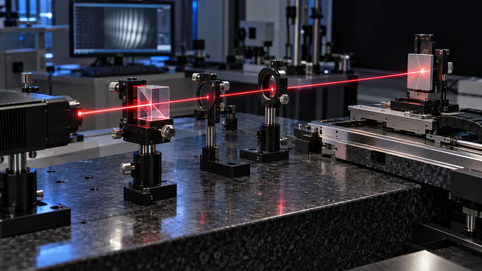
Real axes rarely deviate linearly. Non-linear error compensation addresses this by entering correction values at defined positions across the stroke into a compensation table; the controller interpolates between adjacent points, commonly with linear interpolation. Display and control systems support tables from dozens to hundreds of points per axis, and modern controls allow many compensation values per meter of travel.
The residual error after compensation depends on two things: the spacing of the compensation points and the error shape between them. Encoder manufacturers therefore document the expected residual error after multipoint compensation for specific point intervals—for example, documenting the resulting position error after compensation at 50 mm and 100 mm intervals, where the total error combines the maximum residual error between compensation points with the position error within one signal period.
This framing is the practical takeaway for a machine builder: denser tables reduce the long-range residual but never eliminate the within-period error, which multipoint compensation does not address. The achievable axis accuracy is the sum of both, and the supplier's residual-error data should be part of the selection conversation.
A compensation table is only as good as the measurement behind it. The procedure should stabilize the machine thermally before mapping, use a traceable reference aligned to minimize Abbe offset, approach each target bidirectionally, and repeat the runs to separate systematic error from scatter. Compensation is then computed, entered, and verified with a second measurement.
Multipoint compensation corrects the systematic position error of the measured axis along the measured direction. It does not correct Abbe error caused by the offset between the measuring axis and the working point, because that error changes with straightness and angular motion of the stage and is not fixed by a position table. It does not correct thermal drift that occurs after mapping, reversal error unless it is measured and compensated separately, or dynamic errors that appear only at speed.
It also does not improve the within-signal-period error. That component is set by scale quality, scanning optics and signal processing, and it repeats every period regardless of how dense the compensation table is. Specifying an encoder with a finer signal period or better signal quality is the lever for this part of the budget.
Finally, compensation is attached to a specific configuration. If the scale is replaced, re-mounted, re-spliced or the electronics are changed, the old table describes an axis that no longer exists. Re-measure after any mechanical or electronic change, and schedule periodic verification so drift is caught by data rather than by a failing product.
SENFU treats error mapping as part of system qualification rather than a post-purchase afterthought. For stage projects, the useful conversation starts with the travel, accuracy and repeatability targets, the reference metrology available in the facility, and the environmental conditions under which the compensated accuracy must hold. From there, the map interval, compensation method and verification plan can be defined together.
The same evidence discipline applies on the supplier side: scale accuracy at stated temperature, within-period error, and documented residual error after compensation for the specific configuration. Ask for these as configuration-specific values, because a catalogue figure measured on a different stroke or interval does not predict your axis.
Submit the axis requirement through the application form and SENFU can review it against the encoder family configuration and define the mapping and verification evidence needed before the machine is accepted.
CONCLUSION
Encoder error mapping converts the systematic part of an axis's position error into actionable data: a single ppm factor for a uniform slope, or a multipoint table with interpolation for the real curve. The technique is well established and, applied with a traceable reference and a disciplined procedure, can raise machine accuracy significantly.
Keep the budget honest by adding what compensation leaves behind: residual error between points, within-period error, Abbe offsets, thermal drift and reversal error. With those terms on the table and a verification pass after compensation, the compensated accuracy becomes a measurable, auditable property of the machine.
EVIDENCE CHECKLIST
FAQ
It makes the axis more accurate in the positions and conditions that were mapped, by removing the systematic deviation curve. Residual error between compensation points, within-period error, Abbe offsets and thermal drift remain, so the compensated accuracy is the sum of these terms.
Enough to follow the actual error shape of the axis. If the map shows mostly a straight slope, a linear ppm factor may suffice; if it oscillates, the table should be dense enough that the error between adjacent points is small relative to the target. Controllers support tables from dozens to hundreds of points per axis.
Multipoint compensation addresses position error over the stroke; the error within one signal period repeats too fast for a position table and is set by scale quality, scanning and signal processing. Reducing it requires a finer signal period or better signal quality, not a denser table.
After any change to the scale, its mounting, the electronics or the axis mechanics, after re-splicing or replacing a scale, and periodically as part of machine verification, since thermal history and mechanical wear change the curve over time.
A calibrated, traceable measuring system such as a laser interferometer aligned along the axis of travel, or a comparator measuring system for shorter strokes. The reference uncertainty should be small relative to the compensation target, and the setup should minimize Abbe offset.
Send the travel, accuracy and repeatability targets, expected environment, reference metrology available and the encoder configuration under consideration. SENFU can help define the mapping interval, compensation approach and verification evidence.
AUTHORITATIVE SOURCES
TECHNICAL REVIEW
Send the application, critical parameters and any drawing or process information available.
Discuss your application ↗