
Computed edge frequency
The worst-case output frequency derived from scale pitch or line count and the axis maximum velocity, documented as a design input.
TECHNOLOGY / HIGH-SPEED ENCODER FEEDBACK
High-speed counting pushes an optical encoder against several different limits at once: mechanical velocity, interpolation bandwidth, the electrical path and the controller counter. This guide shows how to build the frequency budget and verify it on the real axis.
Published
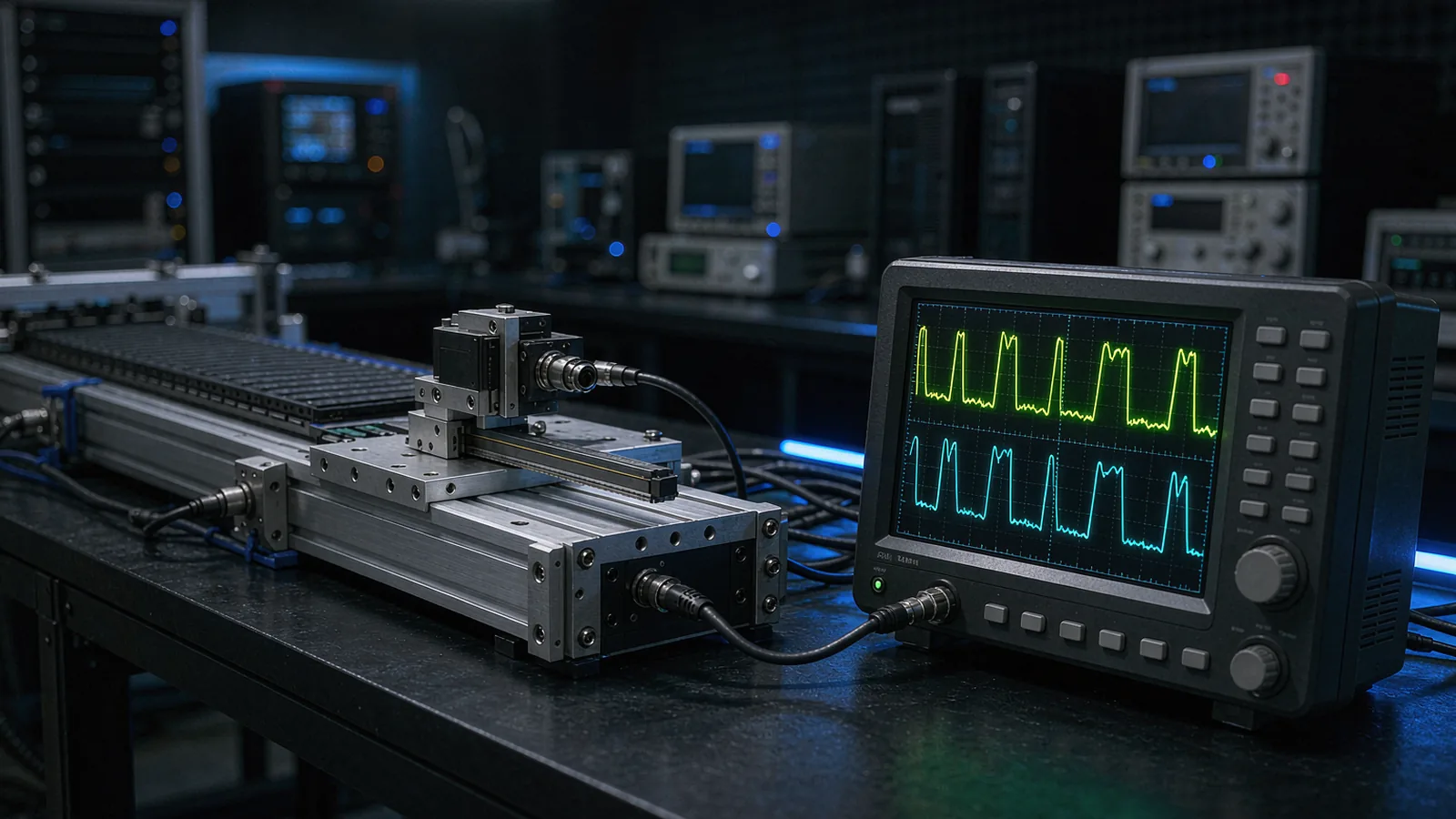
DIRECT ANSWER
An optical encoder's usable counting frequency is set by the whole chain between grating and counter, and no single datasheet number covers it. The output frequency of an incremental channel follows from geometry: scale pitch divided by velocity. A 20 µm pitch scale moving at 2 m/s produces a 100 kHz fundamental, and ×100 interpolation turns that into a 10 MHz edge stream. Each stage in the chain can become the binding limit: the readhead's mechanical velocity rating, the maximum input frequency of the interpolation electronics, the output driver and cable, and finally the controller counter input with its filter settings.
Selection therefore works as a frequency budget rather than a headline figure. Calculate the edge frequency at the axis's worst-case velocity, read the interpolation speed-versus-resolution curve instead of the quoted resolution alone, respect the differential interface and cable length limits, and confirm the counter input toggles reliably at that frequency with the configured glitch filter. Then verify on the real axis by comparing counted displacement against known travel at full speed, because missed counts at velocity rarely appear in slow bench tests.
ENGINEERING CONTEXT
High-speed counting failures are deceptive because the system usually works perfectly at low speed. The integrator sees clean counts during commissioning, then a production axis running at full velocity reports position jumps, lost pulses or occasional reference faults that cannot be reproduced when the machine is stopped. The cause is almost always a frequency limit that nobody budgeted: an interpolator running past its maximum input frequency, an unterminated cable whose edges have degraded into noise, or a counter input whose digital filter silently eats valid pulses. Datasheets contribute to the confusion by quoting resolution, maximum mechanical speed and interface frequency in three different places, each conditional on assumptions the reader rarely sees. The result is equipment selected on compatible numbers that still fails as a system. The fix is to treat counting frequency as a budget computed from the axis's own velocity profile, checked stage by stage, and proven with a counting test at full speed before the machine ships.
Discuss your requirement ↗CRITICAL REQUIREMENTS
The worst-case output frequency derived from scale pitch or line count and the axis maximum velocity, documented as a design input.
The supplier's speed-versus-resolution data confirming the required interpolation factor holds at the working velocity.
Output interface type, cable length limits at frequency, termination recommendation and receiver input specification.
A counting verification at maximum velocity comparing encoder counts against known displacement, with the pass margin recorded.
BUYER MATRIX
Give every shortlisted supplier the same process definition and request configuration-specific proof.
| Limit point | What sets it | Typical symptom when exceeded | How to verify |
|---|---|---|---|
| Readhead mechanics | Maximum velocity rating of the optical head and scale, set by scan frequency and mechanical limits | Signal amplitude collapse or physical damage beyond rated speed | Datasheet velocity rating; check against axis velocity profile including overshoot |
| Interpolation electronics | Maximum input frequency of the analog-to-digital and interpolation pipeline | Resolution silently falls back toward the raw pitch, or periodic position jumps | Supplier speed-versus-resolution curve for the configured interpolation factor |
| Output driver and cable | Driver edge rates, cable capacitance and termination quality | Rounded edges, reflected glitches, counts that drift with cable length or temperature | Oscilloscope at the receiver end at working frequency; differential line check |
| Controller counter input | Counter maximum toggle frequency and digital filter bandwidth | Valid pulses rejected by the glitch filter; counts lag commanded motion | Counter input specification with the actual filter setting; full-speed counting test |
Everything begins with one calculation. For a linear scale, the fundamental signal frequency equals velocity divided by pitch: a 20 µm grating at 2 m/s yields 100 kHz per analog channel. For a rotary ring, line count times revolutions per second gives the same figure. Interpolation multiplies this: ×100 turns 100 kHz into a 10 MHz quadrature pulse train, and a ×4 counter decode raises the edge rate again. The axis's worst case is not its nominal cruise speed but its peak velocity including overshoot, reversal transients and fault stops, so the budget must use the profile the drive can actually produce.
Working the number through the chain stage by stage is what makes high-speed counting predictable. The readhead must be rated for the mechanical speed; the interpolator must accept the fundamental frequency at the wanted factor; the electrical path must deliver edges the receiver can interpret; and the counter must toggle at the resulting rate with its filters configured. A design that only checks one of these four stages has, at best, a quarter of the budget verified.
The interpolation factor that delivers nanometre resolution at low speed cannot always be sustained at high speed. Interpolation electronics need processing time per cycle, so suppliers specify a maximum input frequency beyond which the pipeline either limits the factor or falls back toward the raw scale period. This is why the honest datasheet figure is a curve: resolution as a function of velocity for each interpolation setting. A stage that needs 1 nm resolution for metrology moves but cruises at 1 m/s will typically run two interpolation settings, and the controller must accept the resolution change as the axis accelerates.
Two consequences deserve attention. First, the step size the controller sees changes with velocity, which affects gain scheduling and any compensation that assumes a fixed resolution. Second, exceeding the interpolation input limit does not usually stop the counts; it degrades them, introducing periodic error or jitter exactly at the speeds where the axis spends its production life. The budget should therefore confirm the interpolation setting at the axis peak velocity, not merely at commissioning speed.
A pulse that leaves the readhead perfectly formed can arrive unusable. Square-wave outputs depend on driver edge rates, cable capacitance and termination, and their usable frequency falls as cable length grows, which is why suppliers state cable length limits per interface type. Differential standards such as RS-422 exist precisely for this environment: the differential pair rejects common-mode noise and tolerates longer runs, while single-ended TTL outputs should stay short and well shielded. At megahertz edge rates, unterminated stubs and daisy-chained taps turn the cable itself into a signal integrity problem, and the symptoms—rounded edges, reflected glitches, temperature-dependent miscounts—appear only intermittently.
The receiver side belongs to the same budget. The controller input has its own maximum toggle frequency, hysteresis and digital filter, and a filter width chosen for noise immunity at low speed will reject legitimate high-frequency pulses. Check the input specification with the actual filter configuration, keep the A and B channel pairs length-matched so quadrature phase is preserved, and measure at the receiver end, not at the encoder, when validating with an oscilloscope.
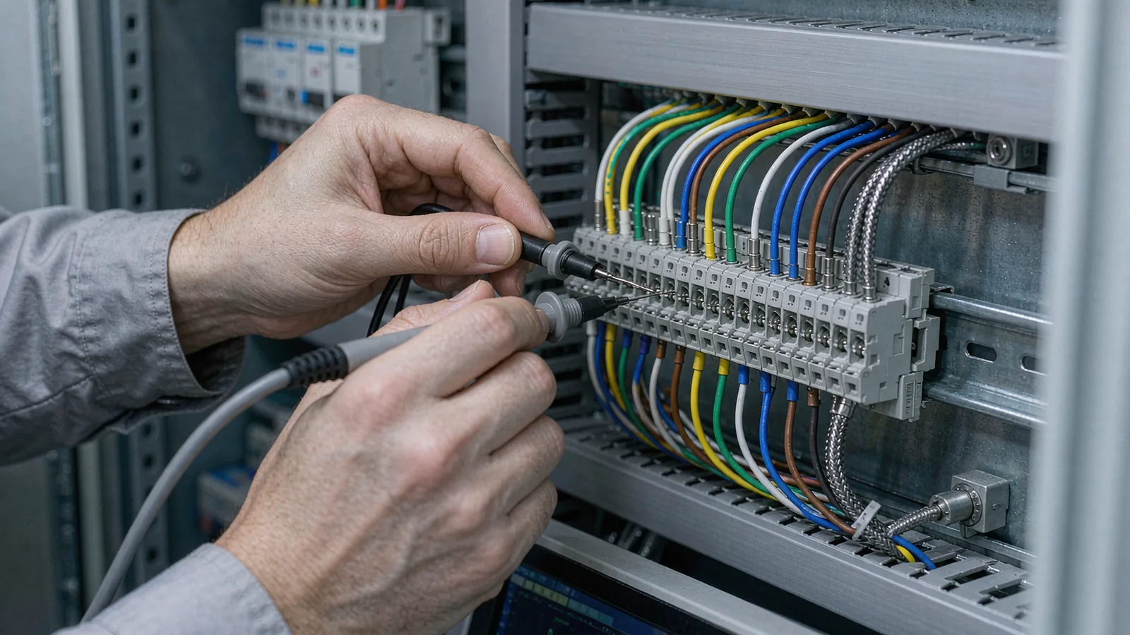
Frequency budgets predict behavior; only a counting test proves it. The core method is simple: command the axis over a known displacement at maximum velocity and compare the counted position against the reference, then repeat bidirectionally and across the speed range. A discrepancy that grows with velocity indicates dropped or spurious counts; a discrepancy that appears only in one direction points to quadrature phase margin. Where absolute reference matters, run the test through the reference mark at speed, because reference capture has its own timing window.
Well-instrumented systems add diagnostics that make marginal counting visible: period monitors that flag implausible pulse spacing, error bits on the interpolation status, and counters that accumulate filter rejections. Record the results as evidence, with the pass margin, because they define the axis's real frequency envelope for future changes to velocity profiles, cable routing or controller firmware. An axis whose counting margin is documented can be modified later without rediscovering the limit.
SENFU publishes speed-versus-resolution data for its readheads and states cable length and interface limits per model, so the frequency budget can be built on real curves rather than assumptions. When an application is submitted with the axis velocity profile, scale pitch options and controller interface, SENFU can confirm the achievable interpolation factor at peak speed and propose the output configuration the counter can actually digest.
For demanding axes, SENFU can also support the counting verification itself, from recommended test displacements to interpretation of period monitor data, so the installed system is proven at speed before production release.
CONCLUSION
High-speed counting is never limited by a single number. Mechanical velocity, interpolation bandwidth, the electrical path and the counter input each impose a ceiling, and the axis runs at the lowest of them. Computing the edge frequency from pitch and peak velocity, then checking it against each stage with the supplier's actual curves, turns an intermittent production fault into a design constraint handled on paper.
Close the loop with a full-speed counting test that compares counted displacement against known travel, and keep the pass margin in the machine documentation. An encoder chain selected and verified this way delivers its headline resolution where it matters—at production speed—rather than only on the bench.
SOLUTION ROUTES
EVIDENCE CHECKLIST
FAQ
For a linear scale, divide velocity by signal period: a 20 µm pitch scale at 2 m/s gives a 100 kHz fundamental per analog channel. Multiply by the interpolation factor for the pulse train frequency, and remember that a ×4 quadrature decode sets the counter's edge rate. Always use the axis peak velocity, including overshoot, as the input.
Interpolation electronics need a fixed processing time per signal cycle, so beyond a maximum input frequency the interpolation factor is reduced or abandoned. Suppliers document this as a speed-versus-resolution curve; the headline resolution applies only below the corresponding velocity.
Yes. Cable capacitance and imperfect termination slow signal edges and invite reflections, so usable frequency falls as length grows. This is why encoder suppliers state a maximum cable length per interface type, and why differential interfaces such as RS-422 are preferred for long, fast runs.
Usually one of three things: the interpolation electronics running past their input limit, degraded edges at the receiver from cable or termination problems, or a counter digital filter wide enough to reject valid high-frequency pulses. An oscilloscope at the receiver end plus a full-speed counting test separates the cases quickly.
Set the filter from the noise environment, not habit. It must reject the shortest glitch the wiring can produce while passing the shortest valid pulse at peak frequency, which means re-checking the setting whenever velocity, interpolation factor or cabling changes.
Yes. Submit the velocity profile, scale pitch options and controller interface. SENFU can confirm the interpolation factor at peak speed from its published curves, propose the output configuration, and support a full-speed counting verification with documented pass margins.
AUTHORITATIVE SOURCES
TECHNICAL REVIEW
Send the application, critical parameters and any drawing or process information available.
Discuss your application ↗